-
 Sam Calisch authoredSam Calisch authored
Loadcells
Measuring displacement of a point or surface, rather than measuring the deformation of a flexure, offers many possibilities for compact, low-cost load cells. This page gathers some resources on this topic and presents work towards a simple six degree-of-freedom (DOF) loadcell based on these ideas.
Capacitive
One way to determine the proximity of two surfaces is by measuring the capacitance between them. This page documents experiments with a 3 DOF Capacitive load cell using a single printed circuit board.

It is based on a discrete electrostatics solver (shown below), and also documented on the page above.
Magnetic
Another proximity measurement uses the magnetic field instead of the electric field. Integrated circuits are available with extremely sensitive magnetostrictive, magnetorestive, and hall effect sensors. Using differential pairs of these elements, very low-cost, non-contact rotary and linear encoders can be made. A great resource for designing such magnetic devices is the Honeywell Hall Effect Handbook.
AS5510 1 DOF Loadcell
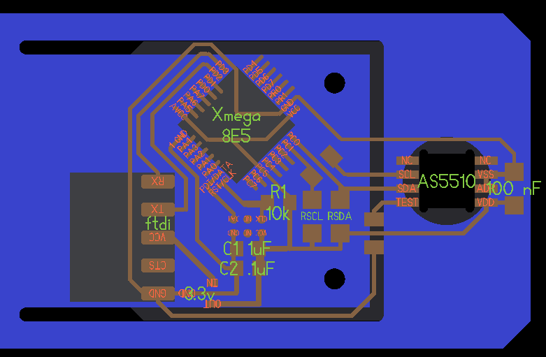
Here, we document experiments with a 1 DOF magnetic load cell, based on the Austrian microsystems AS5510 10 bit linear encoder IC, which boasts 500nm resolution for $1.41 (Q: 100).
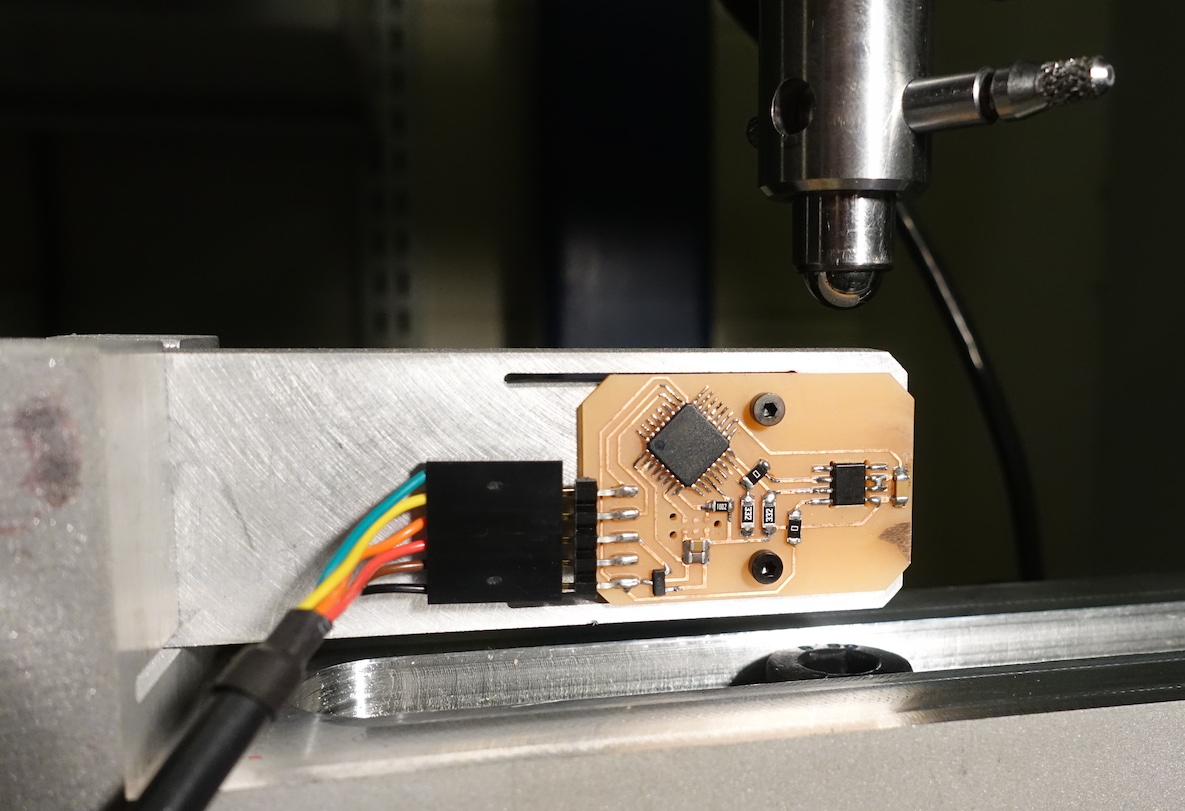
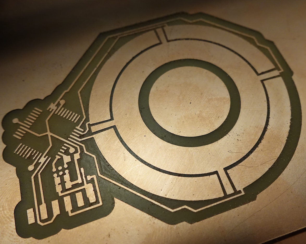
The PCB is mounted to a piece of waterjet aluminum with a flexure cut into it. A magnet sits in a hole on the moving part of the flexure. I designed the flexure to be roughly 5 um/Newton. The encoder wants a air gap of less than 1mm, so I milled away the board inside the SOIC-8 footprint and flipped the part over to bring it closer to the magnet underneath.
I'm using an 8mm circular diametrically magnetized magnet. We could swap in a smaller magnet to push the resolution of the prototype, but I started with the datasheet's recommended magnet form factor. I'm running the chip at its highest sensitivity (+-12.5 mT full scale) and in slow mode (12.5 KHz as opposed to 50 KHz, but .5 mT peak-to-peak noise as opposed to .8 mTpp).
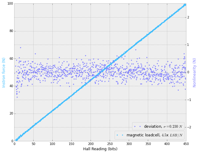
The graphs below show instron characterization of the prototype. First, the flexure had a stiffness of 4.6 um/N, close to the designed 5 um/N. Second, the time series comparison is very boring because the two series are so identical. We see that a displacement of 400 um (corresponding to 100N) takes the encoder nearly over its full range (512 is the full range, as it measures positive and negative displacement to 10 bits (1024)).


Finally, we can plot the relation between the two variables (force and hall reading). Running at the full 12.5 kHz (i.e., without any summing of samples), we get about 5x LSB per Newton. This isn't amazing resolution, but it is very much good enough for my application. Further, we can easily take a hit in speed to get an increase in resolution by summing (i.e., averaging) samples, depending on the applciation.
6 DOF Loadcell
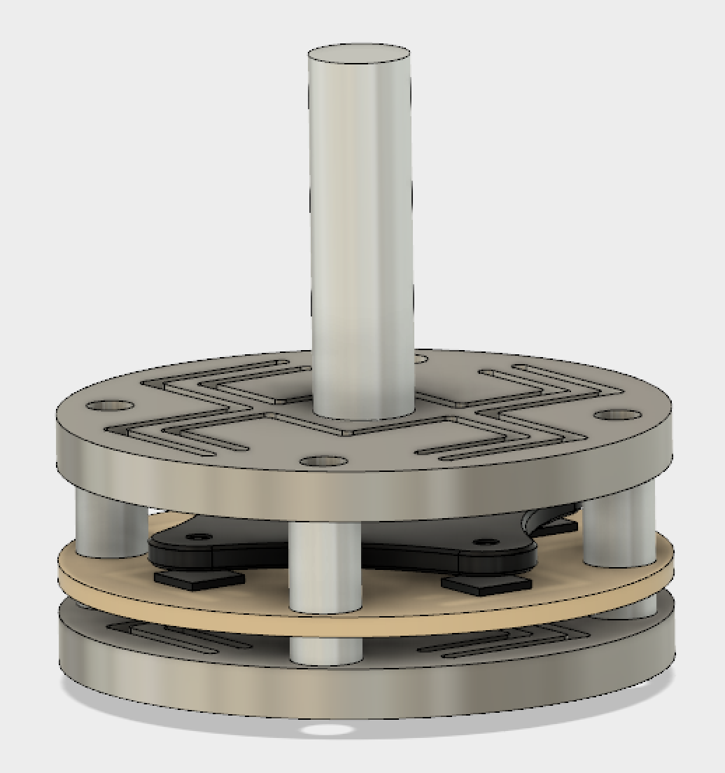
A concept for a 6 degree of freedom magnetic load cell is shown below. It uses a pair of flexures (aluminum or titanium plates on top and bottom) to set relative stiffnesses of Fx, Fy, Fz, Tx, Ty, Tz. A central rod carries a disk with four small neodymium magnets which moves when loads are applied. Four AS5013 hall array ICs are positioned just below the rest positions of the magnets on a single PCB. M3 standoffs and screws hold the entire stack together.
Features of a "good" 6 DOF flexure:
- Ability to tune relative stiffnesses (e.g. Fx/Fz, Tx/Tz, etc.)
- Minimal cross talk (e.g. Fx doesn't induce a displacement in y or a twist, etc.)
- Fits into a reasonably small bounding volume.
Fusion 360 lets us quickly test loading cases for flexure designs. Below are simulations of a force and a moment applied to the loadcell.
Building on the experiments with the AS5510, we explore the use of the AS5013 ($4.42 in Q100) to perform 3-dimensional tracking of a magnet. This IC is nominally an 8-bit 2 axis magnetic encoder, though it contains 5 hall effect sensors, each with 12-bit resolution, adjustable gains, and I2C-accessible raw values. as5013-test/ contains pcb source files for a board to evaluate this measurement.

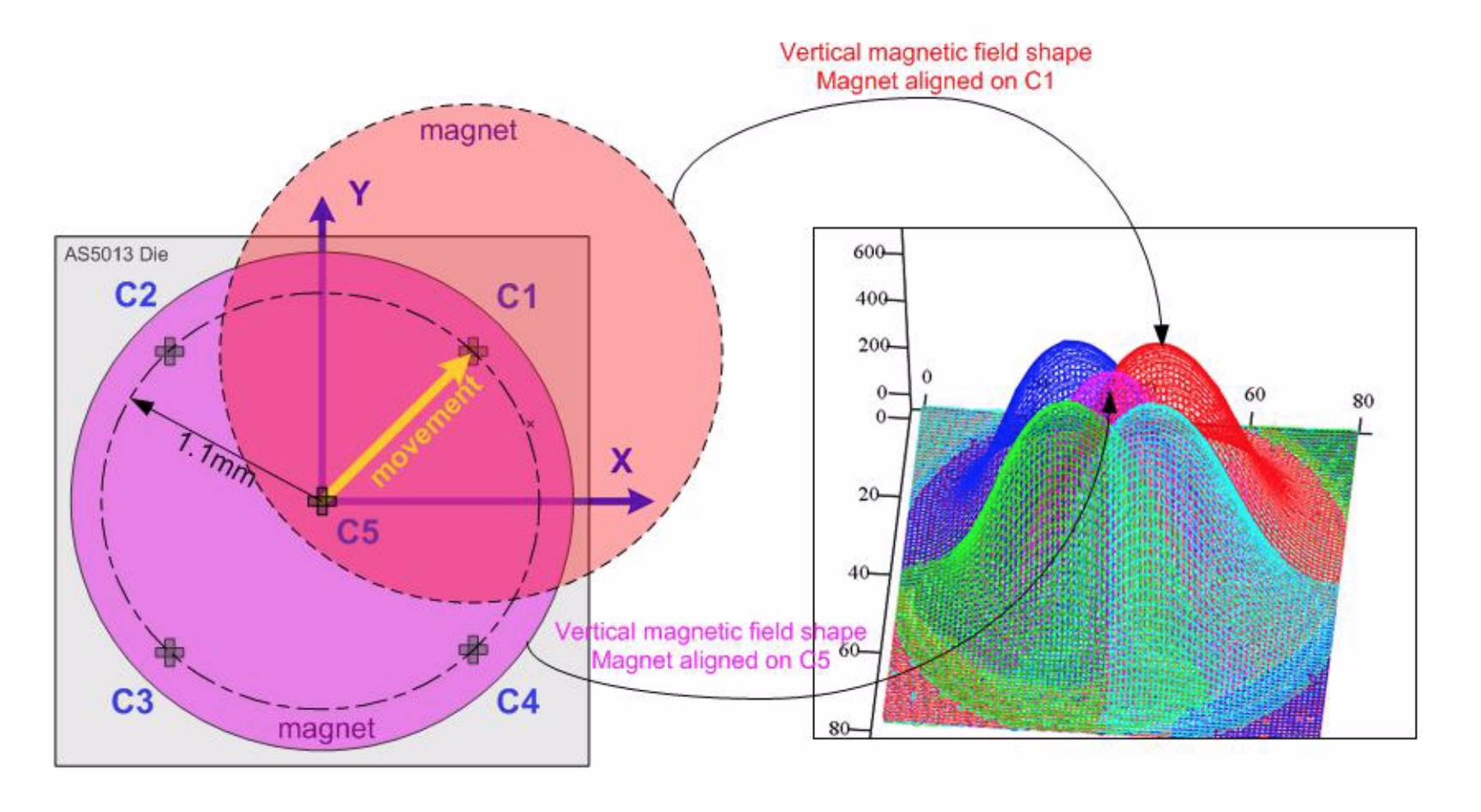
To characterize the use of the AS5013 as a three-dimensional tracking device, we use a 5 axis stage (2 axes motorized, 3 manual) built around two Thorlabs PT1M micrometer stages. After setting a magnet height and orientation, we can sample the 5 hall elements over a two dimensional array of magnet displacements. Executing this for a handful of magnet heights should let us fit functions for X, Y, and Z in terms of the 5 hall readings.


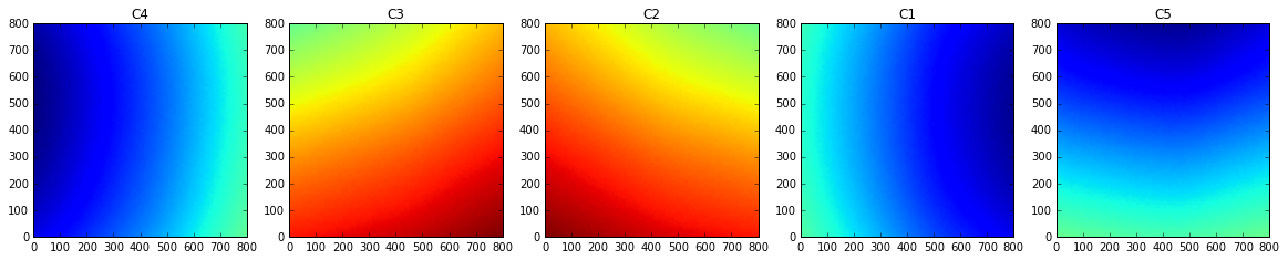
Below are some preliminary plots of readings from the 5 internal hall effect sensors. They each run over 800 um with 10 um sample spacing.
 If we scan over a broader area, we can start to see deviations from an ideal radially symmetric field (there is also an overflow error in these plots that I haven't fixed yet).

This last plot indicates why the magnet spacing is 1.1mm -- from the center of the magnet, this is the approximate distance to the highest gradient in the z component of magnetic field. This observation leads us to consider if we want to maximize resolution in tracking the magnet, could we make an alternative arrangements of magnet(s) to produce higher field gradients.
To test this, I wrote a very simple (and slow for now!) 2D B field finite difference simulation, which is in sim. It uses successive overrelaxation to compute the spatial distribution of the z component of the magnetic field (todo: fix the field magnitude bug here). Below we should output of the simulation for a single magnet, as well as for a pair of opposing magnets. The first plot roughly confirms the shape and size of the magnetic field funtion from a single rod magnet.


The pair of opposing magnets produces a high field gradient. We could create such a region of high field gradient over each of the four outer hall effect sensors using a simple arrangement of square magnets (todo: make a drawing).